THIS IS A DRAFT v1 as of 9 June 2022. Posting it early. Beware of bugs/errors. Will remove this notice once they’re cleaned up. Will also post full code soon.
I present the transformer architecture from ground up in Julia in this post. While my main purpose is to understand it in all detail without relying on any framework, I’m also hoping to try this out a way to teach machine learning … i.e. assuming whole program gradient calculation as a primitive. I won’t be explaining the why of the transformer architecture – for which I refer to Jay Alammar’s awesome tutorial – but mostly the how.
Logistic regression example with Zygote
The Zygote library in Julia provides for whole program differentiation capability which, when combined with Julia’s across library type specialization and optimization facilities, makes for a great toolkit for gradient based ML.
Given a cost function cost() = ... that depends implicitly on parameters
p1, p2 etc. given as vectors or matrices, we can calculate the gradient
of the function w.r.t. the parameters using code like the following –
using Zygote
g = gradient(cost, Params([p1,p2]))
# Then access gradients using the param objects as keys
# g[p1], g[p2], ...
Once you can get hold of the gradient of a cost function, you can run an optimizer and update the parameters based on the calculated gradients to arrive at optimal values for the parameters.
To give a taste of this, let’s start with a simple logistic regression –
using Zygote

# An artificial fake classsifier to mimic
classify(x) = sum(x) < 1.0 ? [1.0, 0.0] : [0.0, 1.0]

# Simple synthetic training data.
x_train = [rand(Float32, 4) for i in 1:20]
y_train = [classify(x) for x in x_train]

# Linear weight matrix and bias
p = (W = rand(Float32, 2, 4),
     b = rand(Float32, 2))

# Predict using parameters.
# In this case, we're calculating cost for the whole
# dataset, but you can modify this same approach for
# batched calculations too (i.e. SGD instead of regular GD)
softmax(x) = let p = exp.(x); p ./ sum(p; dims=1); end

# The main model function
logisticregression(p, x) = softmax(p.W * x .+ p.b)

crossentropy(y, yhat) = -sum(y .* log(yhat .+ 1e-9))
cost() = sum([crossentropy(y_train[i], logisticregression(p, x_train[i]))
             for i in 1:length(x_train)])

# One step of gradient based iteration.
# You just need to keep repeating this until you have
# a good set of model parameters. Optionally, you can use
# available optimizers like ADAM as well.
g = gradient(cost, Params([p...]))
learningrate = 0.01
p.W .-= learningrate * g[p.W]
p.b .-= learningrate * g[p.b]
In the above code, the main model function is logisticregression
and the rest is what we need in order to optimize the parameters
for logistic regression. Given similar x_train, y_train,
and cost function, we can always iterate to get optimal parameters
in this manner.
For the purpose of this post therefore, we’ll focus on the model function and its set of parameters, except that the model function we’ll be building is the transformer.
Julia notation
For the most part, Julia should read like python and be comprehensible as such. There are some specific bits we use here though which could use some explanation.
Broadcasting: If you see a function myfunc called on an array or matrix
like myfunc.(arr), it means “make a new array/matrix by calling that function
on each of its elements.” This also applies to infix operators you’ll encounter
like .+ and .*. In general, the . prefix should give you a clue that
broadcasting is happening. This is not just for special functions provided by
Julia, but is also usable with your own functions, with Julia vectorizing the
calls automatically.
Splatting: If xs is an array of things, then you can use xs... to mean
as though you’d syntactically written xs[1], xs[2], xs[3], ... , xs[length(xs)]. This works in function calls, tuples, array expressions, etc.
Keyword arguments: Unlike python, keyword argument must appear after a
semicolon in function declarations and invocations, within the argument list –
like myfunc(a1, a2; kw1=val1, kw2=val2).
Types are values too: You can store the type of a thing in a named variable
and use that to declare the type of a function argument, and Julia will happily
multiple dispatch over it. You can get the type of a value using typeof(val).
Some basic “layers”
Let’s warm up by constructing some common types of “layers”
of typical neural networks. We’ve already seen one. Just that
we called it logisticregression. This is usually referred to
as a “dense” layer.
There are a few parts to coding up such a layer –
- We need to make a list of parameters that the layer needs.
- We need to implement the layer’s “forward pass”.
- There is no third step … since the gradient computation is handled by Zygote.
Let’s also code up some basic activation functions to start with. We don’t need all of what’s coded below, but they demonstrate how simple functions can be vectorized in julia with no additional effort. These activation functions can be directly used in the network’s code without a framework having to support them through special string constants.
linear(x) = x
sigmoid(x) = 1.0 / (1.0 + exp(-x))
tanh(x) = 2.0 * sigmoid(x) - 1.0
relu(x) = (x < 0.0 ? 0.0 : x)
softrelu(x) = x * sigmoid(x)
To apply one of these activations to a vector or matrix, you just use the
“broadcast” expression .. like softrelu.(x).
The “dense” layer
A utility function to make a matrix of Float32 parameters.
randf32(d...) = rand(Float32, d...) * 2.0 .- 1.0
zerosf32(d...) = zeros(Float32, d...)
mkparams(init, dims...) = init(dims...)
A constructor function to make a named tuple of parameters for our dense layer. We’ll use named tuples for simplicity throughout this post to hold our parameters.
function dense(m, n; activation=relu)
    ( W = mkparams(randf32, m, n),
      b = mkparams(zerosf32, n),
      activation = activation )
end
The first argument is the named tuple of parameters.
The second is the vector or matrix to apply it to.
Note that matrix multiplication in Julia is just *.
const DenseT = typeof(dense(1,1))
feedforward(p::DenseT, x) = p.activation.(p.W * x + p.b)
To pass the second argument to our gradient call, we’ll
also need to be able to extract all our parameters into
an array. We’ll use a params function to help us do that.
Note that our trainable parameters cannot be single numbers
and must be arrays or matrices. If we need single numbers
as trainable parameters, they need to be wrapped into an
array for tracking during gradient calculations.
params(p::DenseT) = [p.W, p.b]
The “dropout” layer
Dropout is also used in the transformer architecture and is one of the simplest layers for regularization. There is one little twist though – dropout layers only kick in at training time and during inference time they’re expected to be no-ops.
function dropout(x; rate=0.8, istraining=true)
    istraining || return x
    scale = 1.0 / (1.0 - rate)
    selected = rand(Float32, size(x)...) .> rate
    scale * (x .* selected)
end
There are no trainable parameters for a dropout layer.
The I/O structure of the transformer
The transformer architecture is posed to solve the problem of machine
translation - where an input sequence in a given language is expected to be
translated into an output sequence in another language. Unlike RNNs, the
transformer network looks at an entire sentence at one shot, for both input and
output. Since sentences can vary in length, the input sequence is considered
with a padding_mask which indicates which words of the input sentence vector
are to be taken into consideration. Output is calculated one word at a time
start from the <SOS> or “start of sentence” token, predicting the next word
assuming that the network has correctly predicted a number of preceding words.
Therefore a portion of the output is masked in order to get the network to
predict the next output word. This mask is referred to as the lookahead_mask.
Instead of using one-hot vectors for the input, we start with a words embedded in a partially semantic space using, say, GloVe embeddings for both the input and output vectors.
The output is calculated using a softmax prediction of the output language’s word index.
So, leaving out hyper parameters of the network, the input-output structure looks like a function of the form –
function transformer(input_sentence, padding_mask, output_sentence, lookahead_mask)
    #...
    return softmax_output
end
Given such a function and the usual crossentropy loss over output minibatches, we can run SGD on the network parameters and train them.
Query, Key and Value
The basic structure of the attention mechanism in the transformer model is built out of three matrices that operate on the input sentence embedding word by word.
-
The “Query” matrix can be thought of as consisting of rows which capture one “question” you can ask of a word such as “Where is this happening?”, “Who is doing this?” and so on.
-
The “Key” matrix then identifies different aspects of words that could serve as answers to the question.
-
The “value” is then a representation that, for each word in the sentence, identifies the role played by that word in answering the question pertaining to one of the other words.
The above is not a strict interpretation and is only offered as an intuition about these matrices.
Position encoding
One of the aspects of the transformer network is that information about relative position between words is encoded as one vector for each position that meets the following criteria –
-
The position of any given word should be uncorrelated with the position of any other word.
-
A “distance” calculated using these vectors between two words separated by k, should largely depend only on k and not on the absolute positions.
The original transformer paper used the following position encoding matrix for a sentence encoded as a matrix of embeddings for each word. Though this was used in the original transformer network, it has recently been shown that even without the position encoding, the network is capable of learning this aspect on its own without significant performance degradation. For the purpose of this post, we’ll stick to the original use of the encoding.
evenfloor(i) = i - (i%2)
position_encoding(i, pos, dk) = sin(pos / (10000^(evenfloor(i)/dk)) + (i % 2) * pi/2)
In the above formula, i ranges over the dk dimensions of the word embedding
and pos ranges over the word indices of the sentence. So we can make a
position encoding matrix using a comprehension like so –
posenc = [position_encoding(i, pos, dk) for i in 0:dk-1, pos in 0:nwords-1]
Basic attention mechanism
So we have three matrices \(W^Q\), \(W^K\) and \(W^V\) that map a given word’s embedding vector into the “query”, “key” and “value” spaces respectively.
The attention calculation tries to answer something like “what is the value corresponding to given query and key, for each word?” by constructing a weighted average of the value space mappings of each word. The weighted average is computed using the following “softmax-like” formula –
$$ \mbox{attention}(q,k,v) = \sum_{i = 1}^{N}{\mbox{softmax}_j(\frac{q_i \cdot k_j}{\sqrt{dk}} + \mbox{mask}_i) \cdot v_i} $$
where
$$
\begin{array}{rcl}
q_i & = & W^Q x_i \\
k_i & = & W^K x_i \\
v_i & = & W^V x_i
\end{array}
$$
In code, that becomes –
# q, k, v are all matrices of dimensions (dk, nwords)
# mask is an array of dimensions (1, nwords) that
# has 1 for included words and 0 for excluded (i.e. masked) words.
# The result is also a matrix of dimensions (dk, nwords).
function attention(q, k, v, mask)
    dk = size(v)[1]
    scale = 1/sqrt(dk)
    if mask == nothing
        v * softmax(scale * (q' * k))
    else
        # The positions where mask has 0 will get mapped to a large
        # negative value, which will end up discounting that position
        # in the softmax calculation.
        emask = -1e6 * (1 .- mask)
        v * softmax(scale * (q' * k)) .+ emask)
    end
end
Multihead attention
The “multihead attention” is an extension of the basic attention mechanism by considering a number of different sets of “questions and considerations” to train for, and combining the output of all of them by mapping each word back into a \(dk\) dimensional space.
We can put together the parameters and calculations like this –
function attention_head(dk, embedding_dimensions)
    ( wq = mkparams(randf32, dk, embedding_dimensions),
      wk = mkparams(randf32, dk, embedding_dimensions),
      wv = mkparams(randf32, dk, embedding_dimensions) )
end

const AttentionHeadT = typeof(attention_head(1,1))

function attention(p::AttentionHeadT, q, k, v, mask)
    attention(p.wq * q, p.wk * k, p.wv * v, mask)
end

function attention(p::AttentionHeadT, x, mask)
    attention(p, x, x, x, mask)
end

params(p::AttentionHeadT) = [p.wq, p.wk, p.wv]

function multihead_attention_layer(nheads, dk, nwords, embedding_dimensions)
    ( head = head(dk, nwords),
      wout = mkparams(randf32, dk, dk * nheads),
      heads = [attention_head(dk, embedding_dimensions) for i in 1:nheads] )
end

const MultiheadAttentionT = typeof(multihead_attention(1, 1, 1))

# p is multihead attention layer parameters
# x is (dk, nwords) given with position encoding.
# mask is (1, nwords) as per description of attention above.
function multihead_attention(p::MultiheadAttentionT, q, k, v, mask)
    attns = [attention(ph, q, k, v, mask) for ph in p.heads]
    attnsmat = cat(attns...;dims=1)
    p.wout * attnsmat
end

function multihead_attention(p::MultiheadAttentionT, x, mask)
    q, k, v = [m * x for m in p.head]
    multihead_attention(p, q, k, v, mask)
end

params(p::MultiheadAttentionT) = vcat(params(p.head), [p.wout], params.(p.heads)...)
The encoder-decoder architecture
We follow the architecture in the original Attention is all you need paper.
So far, in our description of these component functions, we’ve ignored batching. We’ll continue to do that.
The “Add & Norm” layer
The addition is a straight forward residual connection, so we’ll focus on the LayerNorm.
normalizer(dk, nwords) = (scale = mkparams(randf32, dk),
                          bias = mkparams(randf32, dk))

const LayerNormT = typeof(normalizer(1,1))

# Only normalizing over the nwords dimension.
# TODO: Find out whether we should normalize over both dk and nwords.
function layernorm(p::LayerNormT, x; eps=1e-9)
    dk, nwords = size(x)
    mu = sum(x; dims=2) / nwords
    # Shift the mean to 0
    xmu = x .- mu
    # Compute standard deviation to determine scale
    # Note that this is not the bias corrected estimate
    # of the standard deviation (for which we should use nwords-1
    # instead of nwords). It is the oridinary biased estimator.
    d = sqrt.(sum(xmu.^2; dims=2) / nwords)
    n = xmu ./ (d .+ eps) # eps needed to avoid div by zero.
    # Use a "scale layer" on top.
    p.scale .* n .+ p.bias
end

params(p::LayerNormT) = [p.scale, p.bias]
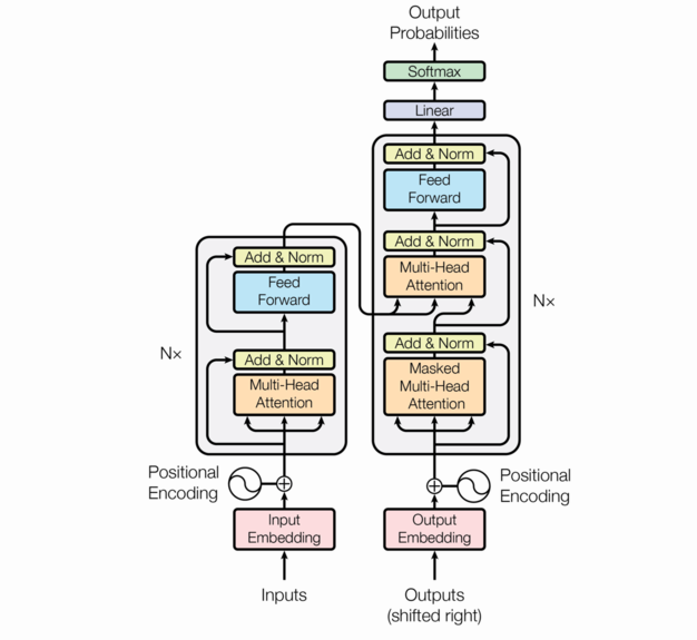
The “encoder”
The picture above shows one block of the “encoder” which is repeated nenc times.
The input to the encoder are the \(q\),\(k\),\(v\) values and each encoder
unit outputs a value for each word as a (dk, nwords) matrix.
A detail that is not visible in the picture is that there is a dropout applied to the following –
- The position encoded input and output vectors
- To the output of every feedforward – i.e. “dense” – layer.
function encoder_unit(nheads, dk, nwords, embedding_dimensions)
    ( mha = multihead_attention_layer(nheads, dk, nwords, embedding_dimensions),
      ff  = dense(dk, nwords; activation=relu)
      norm1 = normalizer(dk, nwords),
      norm2 = normalizer(dk, nwords) )
end

const EncoderUnitT = typeof(encoder_unit(1,1,1))

function encode_one(p::EncoderUnitT, x, mask, dropout_rate, istraining)
    y1 = multihead_attention(p.mha, x, mask)
    y2 = layernorm(p.norm1, y1 .+ x)
    y3 = feedforward(p.ff, y2)
    y4 = dropout(y3; rate=dropout_rate, istraining)
    y5 = layernorm(p.norm2, y4 .+ y2)
    return y5
end

params(p::EncoderUnitT) = vcat(params(p.mha), params(p.ff), params(p.norm1), params(p.norm2))
We now need to stack nenc of these encoder units.
function encoder_stack(nenc, nheads, dk, nwords, embedding_dimensions)
    (encs = encoder_unit(nheads, dk, nwords, embedding_dimensions),)
end

const EncoderT = typeof(encoder_stack(1,1,1,1,1))

function encode(p::EncoderT, x, mask, dropout_rate, istraining)
    y = x
    for enc in p.encs
        y = encode_one(enc, y, mask, dropout_rate, istraining)
    end
    return y
end

params(p::EncoderT) = vcat(params.(p.encs)...)
The “decoder”
The decoder stack is constructed similar to the encoder, except that it operates on the masked output.
function decoder_unit(nheads, dk, nwords, embedding_dimensions)
    (mmha = multihead_attention_layer(nheads, dk, nwords, embedding_dimensions),
     norm1 = normalizer(dk, nwords),
     mha = multihead_attention_layer(nheads, dk, nwords, embedding_dimensions),
     norm2 = normalizer(dk, nwords),
     ff = dense(dk, nwords; activation=relu),
     norm3 = normalizer(dk, nwords))
end

const DecoderUnitT = typeof(decoder_unit(1,1,1))

function decode_one(p::DecoderUnitT, encout, x, mask, dropout_rate, istraining)
    y1 = multihead_attention(p.mmha, x, mask)
    y2 = layernorm(p.norm1, x .+ y1)
    y3 = multihead_attention(p.mha, y2, encout, encout, nothing)
    y4 = layernorm(p.norm2, y3 .+ y2)
    y5 = feedforward(p.ff, y2)
    y6 = dropout(y5; rate=dropout_rate, istraining)
    y7 = layernorm(p.norm3, y6 .+ y4)
    return y7
end

params(p::DecoderUnitT) = vcat(params.(p)...)
And similar to the encoder stack, we make a stack of ndec decoder units.
function decoder_stack(ndecs, nheads, dk, nwords, embedding_dimensions)
    (decs=[decoder_unit(nheads, dk, nwords, embedding_dimensions) for i in 1:ndecs],)
end

const DecoderT = typeof(decoder_stack(1,1,1,1))

function decode(p::DecoderT, encout, x, mask, dropout_rate, istraining)
    y = x
    for dec in p.decs
        y = decode_one(dec, encout, y, mask, dropout_rate, istraining)
    end
    return y
end

params(p::DecoderT) = vcat(params.(p.decs)...)
The output mechanism
Here we capture the last two layers we need in order to get probabilities over the output vocabuluary for each word.
function output_layer(dk, nwords, yvocab)
    ( ff = dense(yvocab, dk; activation=linear), )
end

const OutputT = typeof(output_layer(1,1,1))

function output(p::OutputT, x)
    y1 = feedforward(p.ff, x)
    y2 = softmax(y1)
    reutrn y2
end

params(p::OutputT) = params(p.ff)
Putting it all together
Now we club all of that together into one single transformer function!
function transformer_stack(embedding_dimensions, dk, nenc, ndec, nheads, nwords, yvocab)
    ( enc = encoder_stack(nenc, nheads, dk, nwords, embedding_dimensions),
      dec = decoder_stack(ndec, nheads, dk, nwords, embedding_dimensions),
      out = output_layer(dk, nwords, yvocab),
      hyper = (embedding_dimensions, dk, nenc, ndec, nheads, nwords, yvocab) )
end

const TransformerT = typeof(transformer_stack(1,1,1,1,1,1,1))

function transformer(p::TransformerT, x, y, padding_mask, lookahead_mask, dropout_rate, istraining)
    embedding_dimensions, dk, nenc, ndec, nheads, nwords, yvocab = p.hyper
    posenc = [position_encoding(i, pos, dk) for i in 0:dk-1, pos in 0:nwords-1]
    x = dropout(x .+ posenc; rate=dropout_rate, istraining)
    y = dropout(y .+ posenc; rate=dropout_rate, istraining)

    encout = encode(p.enc, x, padding_mask, dropout_rate, istraining)
    decout = decode(p.dec, y, encout, lookahead_mask, dropout_rate, istraining)
    output(p.out, decout)
end

params(p::TransformerT) = vcat(params(p.enc), params(p.dec), params(p.out))
So … there you go, the transformer network from ground up in Julia!
CAVEAT: I just wrote out this code from top to bottom. I’ve eyeballed it a few times but haven’t tested a single line of it. I will test it though and then update the code with the necessary fixes. However, I hope it was illustrative enough for you to feel confident about how you can just take raw Julia code and, with Zygote, cook up your own ML system, no matter how complex it is.
FluxML: Do also take a look at the awesome FluxML library which provides many of these “layer” types in more flexible form. Here we implemented them for the specific case for illustrative purposes, but usually you’ll reuse code from libraries like FluxML. I also hope that this walk through helps you read some of the internal code of FluxML since the library is essentially built in a similar but more abstract and flexible manner.
- Notations
- Tala Keeper
- Demos
- Talks
GitHub · Twitter · Google+ · LinkedIn · RSS